programming

Manually building manylinux python wheels

After having achived to build the windows wheels for pyLARDA on anacoda, I tried to tackle the linux version. There it’s a bit more complicated, as the wheels are kind of distribution dependent (and are not accepted by pypi).

auditwheel (https://github.com/pypa/auditwheel) allows to put the external shared libraries into the wheel itself, however the have to be compiled with a rather ‘old’ version to be cross-platform compatible.

The manylinux project (https://github.com/pypa/manylinux) providing docker images to simplify this step:

docker pull quay.io/pypa/manylinux2014_x86_64
docker images #to get the id

The source code needs to be available somewhere in the current path, afterwards fire up docker:

docker run -it -v $(pwd):/io 90ac8ec

Then inside the docker container:

cd io/larda
PYBIN=/opt/python/cp38-cp38/bin/
# pyLARDA requires cython as a prerequisite
${PYBIN}/pip install cython
${PYBIN}/pip install .
${PYBIN}/python -m pyLARDA
${PYBIN}/python setup.py bdist_wheel
cd dist/
auditwheel show pyLARDA-3.3.2-cp38-cp38-linux_x86_64.whl
auditwheel repair pyLARDA-3.3.2-cp38-cp38-linux_x86_64.whl

Now the manylinux wheels should be available in the dist/wheelhouse/ directory.


Flexpart 10.4 and GFSv16

My latest encounter with joys of input format change: With the change to GFSv16 in March 2021 additional height levels were added to the grib output. Especially heights below 1hPa. What is generally good news, is bad news for Flexpart 10.4 (as of 20 Nov 2019). The additional levels cause incompatability with the readwinds_gfs.f90. Public information on this issue is rare. There is an Issue in Flexparts ticketing system (https://www.flexpart.eu/ticket/305) but thats more related to the mean-wind trajectory module Flextra.

One suggestion is to drop the additional variables with wgrib2, which is somehow dissatisfying (and I could not figure it out on the short run). The only alternative posed ist, to switch to the dev branch (The link in the issue points to a version 9.3.2 legacy branch). So, for 10.4 dev you want to pull git clone https://www.flexpart.eu/gitmob/flexpart --branch dev --single-branch. With that version, Flexpart switches from grib_api to eccodes, so on ubuntu the libraries apt-get install libeccodes-tools libeccodes-dev are required.

At least for my docker setup, i needed to adapt the makefile:

INCPATH1 = /usr/include
INCPATH2 = /usr/include
LIBPATH1 = /usr/lib
F90 = gfortran

Then, compiling worked sucessfully and the binary could handle the new GFS files.

Slightly related: natural earth cartopy downloads

Seems like the default natural earth mirror is temporarily unavailable (e.g., http://naciscdn.org/naturalearth/110m/physical), but there is this fix: https://github.com/SciTools/cartopy/issues/1298#issuecomment-920843582


FLEXPART 10 into a Docker container

For a recent project, I wanted to include the Lagrangian particle dispersion model FLEXPART (more on that) into an easy-to-deploy project. The analysis part of that project runs on python, but uses some nifty geography libraries, which in turn require C and Fortran libraries. So, I already put this part into a docker container. FLEXPART provides the actual input for the analysis part, so it seemed logical to also include that part.

Not too long ago version 10 came available, also including netCDF output. However, with added dependencies, compiling the source became a bit more complicated. Let’s have a look at the Dockerfile:

FROM ubuntu:18.04


ARG DEBIAN_FRONTEND=noninteractive

RUN apt-get update && apt-get update && apt-get install -y \
  language-pack-en openssh-server vim software-properties-common \
  build-essential make gcc g++ zlib1g-dev git python3 python3-dev python3-pip \
  pandoc python3-setuptools imagemagick\
  gfortran autoconf libtool automake flex bison cmake git-core \
  libjpeg8-dev libfreetype6-dev libhdf5-serial-dev \
  libeccodes0 libeccodes-data libeccodes-dev \
  libnetcdf-c++4 libnetcdf-c++4-dev libnetcdff-dev \
  binutils  python3-numpy python3-mysqldb \
  python3-scipy python3-sphinx libedit-dev unzip curl wget
  
  
# replaced 'libpng12-dev' by libpng-dev
RUN add-apt-repository ppa:ubuntugis/ppa \
  && apt-get update \
  && apt-get install -y libatlas-base-dev libpng-dev \
     libproj-dev libgdal-dev gdal-bin  

RUN add-apt-repository 'deb http://security.ubuntu.com/ubuntu xenial-security main' \
  && apt-get update \
  && apt-get install -y libjasper1 libjasper-dev libeccodes-tools libeccodes-dev

#ENV HTTP https://confluence.ecmwf.int/download/attachments/45757960
#ENV ECCODES eccodes-2.9.2-Source

#
# Download, modify and compile flexpart 10
#
RUN mkdir flex_src && cd flex_src \
  && wget https://www.flexpart.eu/downloads/66 \
  && tar -xvf 66 \
  && rm 66 \
  && cd flexpart_v10.4_3d7eebf/src \
  && cp makefile makefile_local \
  && sed -i '74 a INCPATH1 = /usr/include\nINCPATH2 = /usr/include\nLIBPATH1 = /usr/lib\n F90 = gfortran' makefile_local \
  && sed -i 's/LIBS = -lgrib_api_f90 -lgrib_api -lm -ljasper $(NCOPT)/LIBS = -leccodes_f90 -leccodes -lm -ljasper $(NCOPT)/' makefile_local \
  && make -f makefile_local

ENV PATH /flex_src/flexpart_v10.4_3d7eebf/src/:$PATH

# pip install some more python libraries

The interesting part happens in L34-42. The source is downloaded and unpacked. Then the makefile  needs to be modified to find all libraries (which were installed with apt-get before). Sed is of great use here. First a line is added to the makefile_local and another line is searched and replaces. Finally make is executed to compile FLEXPART.

Now the container can be ran and FLEXPART be executed from within. At least for my application with a couple of thousand particles being simulated, performance is sufficient and a small penalty is outweigh by the ease of deployment.

Further reading:

Blue Planet

How much of the Earth’s surface is covered by water? – 2/3 elementary school knowledge. But how to confirm? And what fraction of the southern hemisphere mid-latitudes is covered by ocean?

We need some data first. For a quick shot, the MODIS land cover type classification should be sufficient. MCD12C1 provides global coverage at 0.05° in the HDF4 format. It is a resampled and  stitched together version of the 500m MCD12Q1 version. The user guide provides a nice overview.

Now we need to do some calculations. The python jupyter notebook is on github. The recipe is rather simple: Load the HDF4 dataset, select the IGBP[1] classification, quick plot for visualization, get the projection and the pixel sizes right and finally do some conditional sums.

The projections and the pixel sizes are a crucial point. The dataset is in the MODIS climate modeling grid, which is a geographic lat-lon projection. The pixel area gets smaller towards the poles, which we have to keep in mind, when calculating the size of the per pixel.

Looking at the final numbers, the fraction of water is 71.6%, which is sufficiently close to available estimates. Some discrepancy is expected, as we do not include ice shelfs, sea ice, tides, etc and the underlying resolution is ‘only’ 5km. Barren surfaces cover around 4.0% of the Earth (13.9% of the land) and ice sheets, including permanent snow cover 2.9% (10.2% of the land).

When splitting up the hemispheres, in the Northern Hemisphere water covers 61.4%, barren 7.5% and ice less than 1%. Of all the land, barren surfaces cover 19.4%. In the Southern Hemisphere, water makes up 81.8% of the surfaces, with barren less than 0.5% and ice 4.8%.

Finally the mid-latitudes. As a rather crude definition, the latitudes between 30° and 70° are used. In the northern mid-latitudes water covers 48.0% (5.7% barren and 0.7% ice). Barren surfaces make up 11.0% of the land. The southern mid-latitudes are overwhelmingly covered with water (93.9%, barren <0.2%, ice 1.4%).

[1] International Geosphere-Biosphere Programme: http://www.igbp.net/

micro-refactoring: long bool statements

“Hell is other people’s code” – while trying to reprocess some data on our server, a colleagues script did not produce the desired output. The problem was, that the location attribute was missing in the input netCDF files [1]. Which leads us to the code, that checked the attributes:

#next the formatting I'm supposed to check it against:

(key_for_range_dimension,key_for_time_dimension,key_for_azimuth_variable,key_for_elevation_variable,key_for_range_variable,key_for_unix_time_variable,key_for_doppler_velocity_variable,key_for_doppler_velocity_error_variable,key_for_nyquist_velocity_variable)=variable_name_key_setting_function(location_we_want,system_we_want,location_info,formatting_translator_dictionary,verbose)
       
#this is a logical statement that includes everything, using brackets to break up inline statements and make it easier to see
formatting_is_correct=(
               'location' in that_files_attributes
               ) and (
                              'system' in that_files_attributes
                              ) and (
                                            key_for_range_dimension in that_files_dimensions
                                            ) and (
                                                           key_for_range_variable in that_files_variables
                                                           ) and (
                                                                         key_for_time_dimension in that_files_dimensions
                                                                          ) and (
                                                                                        key_for_unix_time_variable in that_files_variables
                                                                                        ) and (
                                                                                                        key_for_azimuth_variable in that_files_variables
                                                                                                        ) and (
                                                                                                                       key_for_elevation_variable in that_files_variables
                                                                                                                       ) and (
                                                                                                                                     key_for_doppler_velocity_variable in that_files_variables
                                                                                                                                     )

print("Check format keys:")
print(('location' in that_files_attributes),
    ('system' in that_files_attributes),(key_for_range_dimension in that_files_dimensions),
    (key_for_range_variable in that_files_variables),(key_for_time_dimension in that_files_dimensions),
    (key_for_unix_time_variable in that_files_variables),
    (key_for_azimuth_variable in that_files_variables),
    (key_for_elevation_variable in that_files_variables),
    (key_for_doppler_velocity_variable in that_files_variables))

[You might want to expand the code snippet to fully appreciate the >380 column lines]

At least for me, that looked like a classical broken window. The final print statement is already a owned to the debugging efforts. Two points, that I consider problematic:

    1. insanely long lines (not the only occurrence in that script but a prominent one)
    2. the long and nested boolean statement

Both make it hard to understand, debug and modify the code. Let’s have see, what we quickly can do about it.

var_name_key_setting = variable_name_key_setting_function(
               location_we_want, system_we_want, location_info,
               formatting_translator_dictionary, verbose)
# unpack the function return
(key_for_range_dimension, key_for_time_dimension, 
 key_for_azimuth_variable, key_for_elevation_variable, 
 key_for_range_variable, key_for_unix_time_variable, 
 key_for_doppler_velocity_variable, 
 key_for_doppler_velocity_error_variable,
 key_for_nyquist_velocity_variable) = var_name_key_setting
       
formatting_is_correct_list = [
    'location' in that_files_attributes, 
    'location in attributes',
    'system' in that_files_attributes, 
    'system in attributes',
    key_for_range_dimension in that_files_dimensions, 
    'key range dim in files_dimensions',
    key_for_range_variable in that_files_variables,
    'key range var in files_variables',
    key_for_time_dimension in that_files_dimensions,
    'key time dim in files_dimensions',
    key_for_unix_time_variable in that_files_variables,
    'key unix_time_var in files_variables',
    key_for_azimuth_variable in that_files_variables,
    'key azimuth var in files_variables',
    key_for_elevation_variable in that_files_variables,
    'key elevation var in files_variables',
    key_for_doppler_velocity_variable in that_files_variables,
    'key doppler_vel_var in files_variables',
       ]
formatting_is_correct = all(formatting_is_correct_list[::2])

print("Check format keys:", formatting_is_correct)
if not formatting_is_correct:
       [print('  ', e[0], e[1]) for e in \
            zip(formatting_is_correct_list[0:-1:2], 
                formatting_is_correct_list[1::2])]

Still not perfect, but a bit more explicit and easier to read. In fact the [::2] could also be omitted, as a string also evaluates to True in all().

Maybe it’s time to setup a compulsory linter or at least make PEP 8 and the Google Python Style Guide required reading.

[1] actually required a second pair of eyes to figure out…

SELinux, systemd and python virtual environments

Recently I wanted to configure a gunicorn backend at our newest server. The aim was to run a flask-based python application using a virtual environment in a users home. The machine is running recent Red Hat 8 and the setup of systemd was straightforward and well documented in the internet (e.g. here). However, after

systemctl daemon-reload
systemctl enable ourservice
systemctl start ourservice

a strange permission denied error occurred (also journalctl helps in that context).

After rechecking the file permission several times I finally remembered, that Red Hat now runs runs SELinux. It allows even finer access control for files, resources and actions using policies. The current status of SELinux can be shown with sudo sestatus. For testing reasons, all policies can be set to permissive using sudo setenforce permissive. The contexts of a file can be inspected with ls -Z file1.

To debug an process that fails, the /var/log/audit/audit.log file is the first place to look at. The audit2why tool translates the error messages to a more understandable format:

>
sudo cat /var/log/audit/audit.log | grep gunicorn | audit2why

Afterwards the audit2allow utility can generate rules, that would allow the denied operations:

>
sudo cat /var/log/audit/audit.log | grep gunicorn | audit2allow -M custom_rule

These rules are now stored in the format of an type enforcement (custom_rule.te) file and a policy package which can be activated using semodule -i custom_rule.pp.

Likely this process has to be repeated, as different kinds of operations might be denied.

For our setup the final type enforcement file looked like

module custom_rule 1.0;
 
require {
        type init_t;
        type unconfined_exec_t;
        type user_home_t;
        class file { append execute execute_no_trans ioctl map open read setattr };
        class lnk_file { getattr read };
}
 
#============= init_t ==============
#!!!! This avc is allowed in the current policy
allow init_t unconfined_exec_t:file { execute open read };
allow init_t user_home_t:file setattr;
 
#!!!! This avc can be allowed using the boolean 'domain_can_mmap_files'
allow init_t user_home_t:file map;
 
#!!!! This avc is allowed in the current policy
#!!!! This av rule may have been overridden by an extended permission av rule
allow init_t user_home_t:file { append execute execute_no_trans ioctl open read };
 
#!!!! This avc is allowed in the current policy
allow init_t user_home_t:lnk_file { getattr read };

The type enforcement rule can be compiled manually

checkmodule -M -m -o custom_rule.mod custom_rule.te
semodule_package -o custom_rule.pp -m custom_rule.mod
sudo semodule -i custom_rule.pp
Further useful resources
 
Disclaimer

When used correctly, SELinux adds a lot to your server’s security. When you run into problems with certain commands being denied, you should first make sure that you truly understand what causes the error. Chances are very high that SELinux complains for a reason. Often you can avoid the problem altogether by rethinking where you put which files. When you are absolutely sure that you need to build a new policy package, do yourself a favor and research thoroughly what each added rule does – it is only too easy to create security holes which would defeat SELinux’ purpose.

Michael Trojanek: How to compile a SELinux policy package

UPDATE

Master’s Thesis: Lessons Learned

Now, after finishing my master’s thesis, i would like to recap some experiences i made while working on it. Special emphasis will be put on the programming/data analysis aspect. The core of the thesis is a software called spectra mole, that combines Doppler spectra data from different active remote sensing instruments (Radar and Lidar) with the aim to observe vertical air motion inside clouds.

Language

This is kind of an endless discussion. Popular choices within the field, regarding interpreted/scripting/data analysis languages are: Matlab, IDL, R, Labview and Python
Endless arguments are held which one is superior to others, here are some reasons why I choose Python: it is open source (compared to Matlab, IDL and Labview) and a general purpose language (compared to R. It is not that much fun to do a plain Fourier transform with a statistics language). There are hundred thousands of tutorials available and nearly every question was already asked on stackoverflow.

Modularity and Unit Testing

One major issue in writing scientific software is, that you have to assure that your calculations are correct. With increasing length and complexity of the algorithm, this becomes more and more difficult. The standard software development approach is to separate the program into small independent parts, that can be tested on their own.
The first version of my software was more or less divided into separate units, but without clear interfaces. So the units were quite entangled, which made testing nearly impossible. Refactoring was inevitable. Instead of generating one object and accessing the data at will, now a dictionary containing the data is passed from method to method (making this the “clear” interface). For each method a test case is implemented using pytest. This brought me a huge step forward in terms of reliability of the software.

Layers

Connected to the modularity topic is a layered design. This means that different levels of abstraction and processing steps are separated. For spectra mole this means, that data loading is separated from the processing and all auxiliary data is provided by separate modules.  All post processing (mostly long term statistics) is done after a defined interface, which is in my case an output file.

Version Control/Source Code Management

Its a good idea to keep track of your source code history. The de-facto standard tool for that is git (besides maybe mercurial). One advantage is, that there are a bunch of tutorials and additional tools available. To name a few: github, bitbucket,GitKraken, etc.
Using version control, was a decision I made quite early, and it was a good one.

Visualization

Fast and easy plotting of the data can be quite helpful during development. The plotting routine is always a trade-off between flexibility, usability and quality (respectively beauty). The one tool for all purposes is hard to achieve.

Tracking

The general workflow is to write a chunk of analysis software, run it on some data and look at this data. If any quirks or points for improvement are found, they are implemented and the cycle starts again. Within this process it is necessary to track which version of the software was used on what data. This includes the settings used for each run. Such settings can be for example smoothing lengths, methods used, etc. Ideally they are saved in a machine readable text file using a markup language like json, toml or yaml.

For the software a source code management tool (see above) does this job quite well. But you should consider putting the text-files containing settings under version control, too. For the data itself i have found no solution, that works for me. Maybe saving the commit identifier of the used software version…

This leads to another point: the automation of the whole process.

Automation

Full tacking is possible, when the whole data modification/evaluation chain is automatized. This means, that all parameters and settings are stored in config files and all subroutines are called from one script. Even a simple shell script is enough. Of course this script and the config files should be version controlled.

When it becomes necessary, reprocessing can be done by going back to the old commit and running the script again.

Most of the progress in scientific programming is achieve in an iterative way, i.e. a small part of the code or a setting is changed and the data is reevaluated. Hence, it is in the responsibility of the programmer to “safe” his progress after each significant step.

Final thought

As most applied scientists, I received no extensive formal training on computer science and software development. It takes quite an effort to obtain these skills on your own and write software, that meets at least the most basic quality standards. One book that I can recommend in this context is “The Pragmatic Programmer: From Journeyman to Master” (ISBN: 978-0201616224).

Update 2019-12-14:

Googling the books title, you will likely find a downloadable version of the book.

Unit Tests in Scientific Programming

Testing your code seems like a sane idea, at least from a programmers perspective [eg 1]. As a scientist when it comes to crunching numbers, in the majority of cases, you hack together a small script and hope that it runs as intended. If strange behavior (aka bug) occurs while processing a gigabyte large dataset, you give it a quick fix, pray for the best and start computation all over. After nights of debugging it gets clear that this is not the best approach (or earlier  – i have learned it the hard way).

Assuring the correct execution is rather easy for small parts of code. It is obvious what the following (exaggerated simple) function does:

def larger_zero(number): 
    return number > 0

Problems develop with increasing length of the function or multiple functions/objects interacting with each other. In the real world you are more likely to have a ~1000-lines-of-code data analysis script. It is reading from different files, doing computations and plotting and finally writes the results out. How to assure correct execution in this case?

When your scientific software is modularized (which it ideally is, but this topic is too broad to discuss it here), testing seems pretty straightforward:

  1. starting at the bottom: test independent functions on their own (the core of unit testing)
  2. make sure, that the communication between functions works correct
  3. examine if the whole script does what you intended

Some people argue, that you should write the tests before you start to write your software. In science where you might not know at the beginning what your program should look like at the end, this is not the perfect solution. My current way to go, looks approximately like this (I’m not claiming that there is no room improvements):

  • play with the problem, get an idea about the structure of your program
  • draft (and maybe write) the tests
  • write the actual software, unit test regularly
  • if you encounter a bug, write a test reproducing this bug, then debug
  • test on a larger scale (for example with a test dataset – if there is one)
  • give it a try with the real data (remember: bug -> test to reproduce -> fix the bug)

But enough with the theory, lets look at a simple example. As I am still a novice in the field of (unit) testing, don’t expect too much 😉 Python is the language of my choice for scientific tasks [2]. Aside from unittest (included in the python standard library), pytest [3] seems a good library to get started with unit testing. Installation is straightforward using pip. To illustrate the case I will use a (slightly simplified) piece of code written during my master’s thesis. The quality_mask() function is used to categorize measurements based on quality criteria.

from __future__ import print_function
import numpy as np

def quality_mask(data):
    """ """
  
    if data['Zcr'] > -25. and (data['LDRcr'] < - 14 or np.isnan(data['LDRcr'])):
        print('# particle influenced')
        flag = 1

        if data['momentswp'][0][0] < -29.:
            #print('# low reflectivity')
            flag = 2

        if data['momentswp'][0][1] < data['vcr']:
            # left of cloud radar and above convective boundary layer
            flag = 6

            if (len(data['momentswp']) > 1
                and data['momentswp'][1][1] > data['vcr']
                and data['momentswp'][1][0] > -29.):
                flag = 4

        if len(data['momentswp']) > 6 \
                and data['momentswp'][4][0] > -30.:
            # print('# too many peaks (melting layer)')
            flag = 5

        #if snr_main_peak < 20.:
        if data['SNRwp'] < 15.:
            # print('# low snr')
            flag = 3

    elif data['LDRcr'] > - 14. and data['Zcr'] > 0.:
        # melting layer
        flag = 5
        
    else:
        # not particle influence
        flag = 0
        
    return flag

As there are several input parameters and a lot if-conditions you want to get sure, that classification works as expected. This calls for a unit test. It can be located in a separate file, to keep things clean. Each test has its own data dictionary and checks for the correct output.

from __future__ import print_function
import numpy as np

def quality_mask(data):
    """ """
  
    if data['Zcr'] > -25. and (data['LDRcr'] < - 14 or np.isnan(data['LDRcr'])):
        print('# particle influenced')
        flag = 1

        if data['momentswp'][0][0] < -29.:
            #print('# low reflectivity')
            flag = 2

        if data['momentswp'][0][1] < data['vcr']:
            # left of cloud radar and above convective boundary layer
            flag = 6

            if (len(data['momentswp']) > 1
                and data['momentswp'][1][1] > data['vcr']
                and data['momentswp'][1][0] > -29.):
                flag = 4

        if len(data['momentswp']) > 6 \
                and data['momentswp'][4][0] > -30.:
            # print('# too many peaks (melting layer)')
            flag = 5

        #if snr_main_peak < 20.:
        if data['SNRwp'] < 15.:
            # print('# low snr')
            flag = 3

    elif data['LDRcr'] > - 14. and data['Zcr'] > 0.:
        # melting layer
        flag = 5
        
    else:
        # not particle influence
        flag = 0
        
    return flag

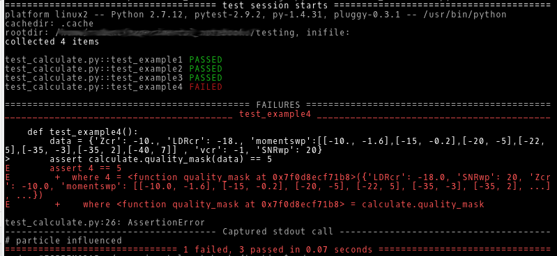
Now we are ready to run the test with  py.test -v test_calculate.py. The output looks like this:

unittest_outputThe first three test passed nicely. The forth one fails, either caused by a bug in the function or – in this case – an error in the data used for that test.

Furthermore the test procedure is very fast: 0.07s. You can use it frequently during and after coding, to ensure code quality without loosing too much time. Many professional teams run their tests every time they commit to their repository or even automated during the night.

Further reading