Master’s Thesis: Lessons Learned

Now, after finishing my master’s thesis, i would like to recap some experiences i made while working on it. Special emphasis will be put on the programming/data analysis aspect. The core of the thesis is a software called spectra mole, that combines Doppler spectra data from different active remote sensing instruments (Radar and Lidar) with the aim to observe vertical air motion inside clouds.

Language

This is kind of an endless discussion. Popular choices within the field, regarding interpreted/scripting/data analysis languages are: Matlab, IDL, R, Labview and Python
Endless arguments are held which one is superior to others, here are some reasons why I choose Python: it is open source (compared to Matlab, IDL and Labview) and a general purpose language (compared to R. It is not that much fun to do a plain Fourier transform with a statistics language). There are hundred thousands of tutorials available and nearly every question was already asked on stackoverflow.

Modularity and Unit Testing

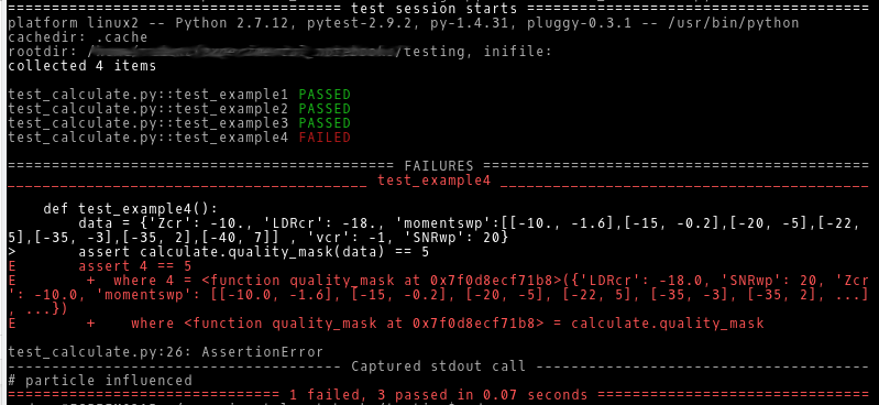
One major issue in writing scientific software is, that you have to assure that your calculations are correct. With increasing length and complexity of the algorithm, this becomes more and more difficult. The standard software development approach is to separate the program into small independent parts, that can be tested on their own.
The first version of my software was more or less divided into separate units, but without clear interfaces. So the units were quite entangled, which made testing nearly impossible. Refactoring was inevitable. Instead of generating one object and accessing the data at will, now a dictionary containing the data is passed from method to method (making this the “clear” interface). For each method a test case is implemented using pytest. This brought me a huge step forward in terms of reliability of the software.

Layers

Connected to the modularity topic is a layered design. This means that different levels of abstraction and processing steps are separated. For spectra mole this means, that data loading is separated from the processing and all auxiliary data is provided by separate modules.  All post processing (mostly long term statistics) is done after a defined interface, which is in my case an output file.

Version Control/Source Code Management

Its a good idea to keep track of your source code history. The de-facto standard tool for that is git (besides maybe mercurial). One advantage is, that there are a bunch of tutorials and additional tools available. To name a few: github, bitbucket,GitKraken, etc.
Using version control, was a decision I made quite early, and it was a good one.

Visualization

Fast and easy plotting of the data can be quite helpful during development. The plotting routine is always a trade-off between flexibility, usability and quality (respectively beauty). The one tool for all purposes is hard to achieve.

Tracking

The general workflow is to write a chunk of analysis software, run it on some data and look at this data. If any quirks or points for improvement are found, they are implemented and the cycle starts again. Within this process it is necessary to track which version of the software was used on what data. This includes the settings used for each run. Such settings can be for example smoothing lengths, methods used, etc. Ideally they are saved in a machine readable text file using a markup language like json, toml or yaml.

For the software a source code management tool (see above) does this job quite well. But you should consider putting the text-files containing settings under version control, too. For the data itself i have found no solution, that works for me. Maybe saving the commit identifier of the used software version…

This leads to another point: the automation of the whole process.

Automation

Full tacking is possible, when the whole data modification/evaluation chain is automatized. This means, that all parameters and settings are stored in config files and all subroutines are called from one script. Even a simple shell script is enough. Of course this script and the config files should be version controlled.

When it becomes necessary, reprocessing can be done by going back to the old commit and running the script again.

Most of the progress in scientific programming is achieve in an iterative way, i.e. a small part of the code or a setting is changed and the data is reevaluated. Hence, it is in the responsibility of the programmer to “safe” his progress after each significant step.

Final thought

As most applied scientists, I received no extensive formal training on computer science and software development. It takes quite an effort to obtain these skills on your own and write software, that meets at least the most basic quality standards. One book that I can recommend in this context is “The Pragmatic Programmer: From Journeyman to Master” (ISBN: 978-0201616224).

Update 2019-12-14:

Googling the books title, you will likely find a downloadable version of the book.

Impressionen Schwerwettertörn Rund Fünen

So, wir sind wieder heil im Binnenland angekommen und inzwischen auch wieder aufgetaut. Ründ Fünen (ab/an Flensburg) hätten wir in 4.5 Segeltagen auch beinahe geschafft, nur die Klappbrücke in Sønderborg konnte uns stoppen.  Wie erhofft, beworben, erwartet waren die Bedingungen “schwer”. Wind von 3 bis 30 Knoten und von Sonnenschein bis Schneeschauer alles dabei. Die Temperaturen waren durchaus herbstlich (irgendwo zwischen 0 und 10ºC) und auch die Infrastruktur war schon in der Winterpause, insbesondere die Sanitäranlagen. Aber dank einer coolen Crew, einem tollem Skipper und einem schnellen Boot (mit Dieselheizung) war es ein unvergesslicher Törn. Zuletzt noch ein kleines bisschen Werbung: Schoenicke skipperteam ist echt zu empfehlen. Alles war kompetent organisiert und sogar der Einkauf war vor unserer Ankunft schon erledigt.

Windstatistik Ostsee im November

[English summary: ERA Interim reanalysis data is used to assemble Pilot Chart like Wind statistics for the western Baltic sea in November.]

Update: Wind in der Ostsee

Anfang November geht es zum letzten Segeltörn dieser Saison: 5 Tage Ostsee ab Flensburg. Um vorab die zu erwartenden Wetterverhältnisse abschätzen zu können bieten sich Monatskarten [1] und die entsprechenden nautischen Veröffentlichungen [BSH, Naturverhältnisse Ostsee 2008] an.

Beide basieren normalerweise auf langjährigen Stations- bzw. Schiffsbeobachtungen mit entsprechenden Nachteilen, wie schlechter Abdeckung abseits von Schifffahrtsrouten, begrenzte Auflösung. Zudem umfassen Unterlagen für die Sportschifffahrt häufig nur die Sommermonate [2]. So eröffnet sich die Frage, ob entsprechende Daten aus numerischen Wettermodellen einen Teil dieser Lücke schließen können.

Daten: ERA Reanalyse

Um für ein Wettervorhersagemodell verwendet werden zu können, muss von Stationsmessungen auf den aktuellen Zustand der Atmosphäre als Ganzs (in Fläche und Höhe) geschlossen werden. Vereinfacht gesagt: Die “Lücken” zwischen einzelnen Messungen müssen geschlossen werden. Dieser komplizierte Prozess nennt sich Datenassimilation. Diese Anfangszustände der Atmosphäre werden in sogenannten Reanalysen gesammelt, um einen einheitlichen Datensatz des “tatsächlichen” Zustands zu erhalten. Diese Reanlysen werden dann unter anderem verwendet, um Modellvorhersagen zu evaluieren. Einen Überblick über die Qualität solcher Reanalysen liefert [3]. Im folgenden wird die ERA-Interim Reanalyse [4] des ECMWF (Europäisches Zentrum für mittelfristige Wettervorhersage) verwendet. Sie umfasst die Daten seit 1979 und wird laufend aktualisiert. Die Auflösung beträgt 3h und 0.5°. Der Datensatz ist frei verfügbar und kann (nach Anmeldung) hier herunter geladen werden [5].

Datenauswertung

Zuerst ist das langjährige Mittel des Windes von Interesse, um die zu erwartenden Bedingungen grundsätzlich einschätzen zu können. Aus dem etwa 6 GB großen Datensatz wird zunächst der November jeden Jahres für ein bestimmtes Seegebiet ausgewählt. Die gesamte Auswertung beruht auf Python mit entsprechenden Bibliotheken (xarray, cartopy, numpy, matplotlib). Bei Gelegenheit stelle ich das aufgeräumte Skript online…

map_southwest_watermark
Zunächst wird nur die süd-westliche Ostsee im rot markierten Bereich berücksichtigt.

Nun wird einfach die relative Häufigkeit der einzelnen Windgeschwindigkeiten bzw. -richtungen berechnet. Im November ist die vorherrschende Süd bis West bei einer mittleren Windgeschwindigkeit von 13.5 kn und Böen von 20 kn. Die mittlere Lufttemperatur im November liegt bei 6.3°C.

wind_summary
Relative Häufigkeit der 3h Maximalböen, der mittleren Windgeschwindigkeit und der Windrichtung.

Im Vergleich mit der Veröffentlichung “Naturverhältnisse in der Ostsee” (BSH, überholte Auflage 1996) sind Windstärken 6-7 Bft (22-34 kn) in dieser Auswertung etwas häufiger, aber der Unterschied ist nicht statistisch signifikant.

In einem Windstern werden die Häufigkeit der Windgeschwindigkeit in Abhängigkeit der Windrichtung dargestellt. Dies ist vor allem in Monatskarten üblich. Hier wird deutlich, dass der Wind am häufigsten aus  S bis W mit 4-5 Bft kommt. Windstärken über 8 Bft kommen vornehmlich aus westlichen Richtugen.

Ausblick

Mit dem gezeigten Ansatz ist es nun ein Leichtes diese Statistik für andere Seegebiete/Monate zusammen zu stellen. In Kürze mehr…

Aber alle Statistik ist geduldig und welche Wetterverhältnisse sich Anfang November 2016 einstellen wird sich zeigen.

Update

Hier noch die Statistik für die angrenzenden Seegebiete. Wie zu erwarten sind die Unterschiede nicht extrem, liegen aber trotzdem im Bereich von 3-5%.

western_baltic_november

Unit Tests in Scientific Programming

Testing your code seems like a sane idea, at least from a programmers perspective [eg 1]. As a scientist when it comes to crunching numbers, in the majority of cases, you hack together a small script and hope that it runs as intended. If strange behavior (aka bug) occurs while processing a gigabyte large dataset, you give it a quick fix, pray for the best and start computation all over. After nights of debugging it gets clear that this is not the best approach (or earlier  – i have learned it the hard way).

Assuring the correct execution is rather easy for small parts of code. It is obvious what the following (exaggerated simple) function does:

def larger_zero(number): 
    return number > 0

Problems develop with increasing length of the function or multiple functions/objects interacting with each other. In the real world you are more likely to have a ~1000-lines-of-code data analysis script. It is reading from different files, doing computations and plotting and finally writes the results out. How to assure correct execution in this case?

When your scientific software is modularized (which it ideally is, but this topic is too broad to discuss it here), testing seems pretty straightforward:

  1. starting at the bottom: test independent functions on their own (the core of unit testing)
  2. make sure, that the communication between functions works correct
  3. examine if the whole script does what you intended

Some people argue, that you should write the tests before you start to write your software. In science where you might not know at the beginning what your program should look like at the end, this is not the perfect solution. My current way to go, looks approximately like this (I’m not claiming that there is no room improvements):

  • play with the problem, get an idea about the structure of your program
  • draft (and maybe write) the tests
  • write the actual software, unit test regularly
  • if you encounter a bug, write a test reproducing this bug, then debug
  • test on a larger scale (for example with a test dataset – if there is one)
  • give it a try with the real data (remember: bug -> test to reproduce -> fix the bug)

But enough with the theory, lets look at a simple example. As I am still a novice in the field of (unit) testing, don’t expect too much 😉 Python is the language of my choice for scientific tasks [2]. Aside from unittest (included in the python standard library), pytest [3] seems a good library to get started with unit testing. Installation is straightforward using pip. To illustrate the case I will use a (slightly simplified) piece of code written during my master’s thesis. The quality_mask() function is used to categorize measurements based on quality criteria.

from __future__ import print_function
import numpy as np

def quality_mask(data):
    """ """
  
    if data['Zcr'] > -25. and (data['LDRcr'] < - 14 or np.isnan(data['LDRcr'])):
        print('# particle influenced')
        flag = 1

        if data['momentswp'][0][0] < -29.:
            #print('# low reflectivity')
            flag = 2

        if data['momentswp'][0][1] < data['vcr']:
            # left of cloud radar and above convective boundary layer
            flag = 6

            if (len(data['momentswp']) > 1
                and data['momentswp'][1][1] > data['vcr']
                and data['momentswp'][1][0] > -29.):
                flag = 4

        if len(data['momentswp']) > 6 \
                and data['momentswp'][4][0] > -30.:
            # print('# too many peaks (melting layer)')
            flag = 5

        #if snr_main_peak < 20.:
        if data['SNRwp'] < 15.:
            # print('# low snr')
            flag = 3

    elif data['LDRcr'] > - 14. and data['Zcr'] > 0.:
        # melting layer
        flag = 5
        
    else:
        # not particle influence
        flag = 0
        
    return flag

As there are several input parameters and a lot if-conditions you want to get sure, that classification works as expected. This calls for a unit test. It can be located in a separate file, to keep things clean. Each test has its own data dictionary and checks for the correct output.

from __future__ import print_function
import numpy as np

def quality_mask(data):
    """ """
  
    if data['Zcr'] > -25. and (data['LDRcr'] < - 14 or np.isnan(data['LDRcr'])):
        print('# particle influenced')
        flag = 1

        if data['momentswp'][0][0] < -29.:
            #print('# low reflectivity')
            flag = 2

        if data['momentswp'][0][1] < data['vcr']:
            # left of cloud radar and above convective boundary layer
            flag = 6

            if (len(data['momentswp']) > 1
                and data['momentswp'][1][1] > data['vcr']
                and data['momentswp'][1][0] > -29.):
                flag = 4

        if len(data['momentswp']) > 6 \
                and data['momentswp'][4][0] > -30.:
            # print('# too many peaks (melting layer)')
            flag = 5

        #if snr_main_peak < 20.:
        if data['SNRwp'] < 15.:
            # print('# low snr')
            flag = 3

    elif data['LDRcr'] > - 14. and data['Zcr'] > 0.:
        # melting layer
        flag = 5
        
    else:
        # not particle influence
        flag = 0
        
    return flag

Now we are ready to run the test with  py.test -v test_calculate.py. The output looks like this:

unittest_outputThe first three test passed nicely. The forth one fails, either caused by a bug in the function or – in this case – an error in the data used for that test.

Furthermore the test procedure is very fast: 0.07s. You can use it frequently during and after coding, to ensure code quality without loosing too much time. Many professional teams run their tests every time they commit to their repository or even automated during the night.

Further reading